Jolt: running Clojure on Chez Scheme
I've been working on a new Clojure implementation targeting Chez Scheme, and it's now at a point where I'd like to share it more broadly in hopes that it might be useful to others. This post will explain the rationale behind the project, its current status, and why it may be of interest.
Why Chez Scheme?
My main goal was to make a drop-in replacement for JVM Clojure which had a fast startup and a light memory footprint. If you look under the hood of Jolt you'll quickly see why Chez Scheme is a great choice for hosting Clojure. Since both languages share the same Lisp roots, the core semantics of Clojure map seamlessly to Scheme, avoiding the impedance mismatch associated with forcing functional paradigms onto something like the JVM. Chez brings a mature JIT compiler to the table that can aggressively optimize the emitted code while maintaining a reasonably small runtime footprint. You also get a highly tuned generational garbage collector that is practically purpose built to handle the rapid allocation and deallocation of immutable data structures inherent to Clojure workflows. Finally, Chez runs natively across a wide variety of operating systems, so you end up getting lean native binaries with instant startup times rather than hauling around a heavy Java environment.
While the JVM is an incredibly powerful piece of engineering, it also happens to be one of the biggest reasons developers cite when passing on Clojure. The Java runtime evolved in an era of enterprise architecture, designed for massive application servers like Tomcat or WebSphere which were effectively their own operating systems. In that model the application server would greedily consume all available host memory and run continuously for months on end, making long JVM startup phases and heavy initial resource footprints perfectly acceptable trade-offs. But that monolithic design clashes with how modern web applications are typically built, especially in fast-paced startup environments where the engineering culture has shifted toward microservices. Today, you typically want to deploy fleets of isolated containers that boot instantly and can dynamically scale horizontally to handle sudden traffic spikes. Hauling around a massive warmed up Java environment just to run a lightweight standalone service goes directly against that principle.
I've always wondered what it would take to create a Clojure runtime that matched modern development practices, and Jolt is my attempt at tackling the problem. There are, of course, already a number of Clojure dialects out there. Jank, in particular, is an effort I'm personally excited to follow. It's already far along toward having a full Clojure implementation, but it focuses on having compatibility with the core language. Unfortunately, most of the existing Clojure libraries end up relying on some interop with the JVM host meaning that they will not run on these dialects without modification.
It would be really nice to be able to leverage the existing ecosystem of mature and battle tested libraries already available, and I was interested to see how feasible it would be to provide Java-specific shims on top of the Chez runtime. My key realization was that most libraries don't actually use much of the Java standard library surface for their interop, and once you map out a few packages like java.io, java.time, and a few others, then you can run a large portion of the current Clojure stack without having to reimplement or port it to the new platform. Again, it's worth noting other efforts such as let-go dialect targeting Go, which is following a similar plan. The key difference is in the platforms we are targeting and the ecosystems they open up access to.
What Works Today
Today, Jolt supports a number of popular Clojure libraries. It is already possible to build a fully fledged Ring app using Ring, Reitit, Selmer, and HoneySQL. The full list of libraries which have their entire test suites passing can be seen on the official documentation site. Some libraries, like Reitit, drop down to Java, but that's not a problem as Jolt makes it possible to provide shims using Jolt libraries. For example, router library implements reitit.Trie Java class needed by Reitit. So, if you need access to a particular Clojure library that doesn't have the shims available in the core language, you can always add them yourself to get them working. In many cases, this doesn't need to be done from scratch either as you can leverage mature Scheme or C libraries for the underlying functionality, and simply write a bit of glue code to expose the functionality as a Java API.
Jolt uses deps.edn for managing dependencies and aliases largely the same way as regular Clojure. As a bonus, you can also specify native C dependencies as seen here. These libraries must be provided on the system in order to be picked up.
The main joy of working with Clojure has always been its interactive development cycle, hence the familiar nREPL workflow is fully supported. You can start a Jolt app, jack in from your favorite editor, and develop it just as you would when running Clojure on the JVM. Additionally, nREPL can be embedded in compiled release binaries as well.
Another thing I wanted to do as part of the project was to map out what actually constitutes Clojure as a spec to follow. So, I'm building out a conformance spec, EBNF, and RFCs, as I add support for existing libraries and discover different quirks along the way. I'd like to give a shout out to clojure-test-suite from the Jank team which has been invaluable for getting bootstrapped and having confidence that core language semantics such as the reader, the special forms, and the bulk of clojure.core are correct. However, it stops short of the JVM host contract that many libraries depend on, so most of the effort in building the corpus went into closing that gap. It sources every expected value from reference JVM Clojure and currently holds around 3,500 cases, each tagged as either portable (:common, something any faithful Clojure dialect must satisfy) or host-dependent (:jvm, exercising interop). A certification step re-evaluates the whole corpus against real Clojure to catch unclassified divergences, ensuring that the contract doesn't quietly drift.
Under the Hood
Getting libraries to work surfaced a recurring set of problems. On the host side, Jolt mirrors nine java.* packages commonly used by popular Clojure libraries. These include java.io, java.lang, java.util, java.time, java.math, java.net, java.nio, java.sql, and java.text with roughly a thousand method and field implementations across those packages. It's worth noting that Jolt doesn't provide a full reimplementation of the JVM standard library. While most of these classes carry complete method sets, a few resolve only enough for instance? and type checks to land correctly, and a handful like bean and proxy are documented partials. In a lot of cases, it's enough that interop forms like Math/sqrt, (StringBuilder.), and instance? resolve against real behavior rather than needing to plumb out a true class hierarchy.
With no JVM underneath, class identity has to be synthesized using a hierarchy graph to back instance? and (class x), and raw Chez runtime errors need to be mapped onto a faithful JVM exception hierarchy so that catch dispatch can work correctly. The cases that plain value-equality can't catch were the trickiest to get right here. For example, the whole seq producer family has to be lazy at construction, realize left to right, memoize, and chunk in 32-element runs to match what Clojure does, while the numeric tower requires full JVM contagion rules plus 64-bit wrapping for unchecked math. The real test, though, was simply running the real test suites for individual libraries to discover subtle implementation quirks and Java host interactions. Porting spec.alpha, core.logic, core.async, test.check, tools.reader, rewrite-clj, and a few dozen others shook out most of the edge cases like data readers returning code forms, namespaced-map literals, *print-length* and *print-level*, protocol methods merging across deftype and reify, and even soft and weak references with genuine GC eviction wired through Chez's weak pairs and guardians.
In terms of footprint, a minimal binary compiles to around 13 megs without optimizations and just 8 megs when direct linked. When it comes to actual performance, Jolt is currently comparable with JVM Clojure in a number of benchmarks having parity or being around 2x slower on most, while only being around 7x worse in a couple of cases. This was made possible entirely by the mature Chez runtime. And, of course, just as we can drop down to Java with regular Clojure, Jolt lets you do the same with Scheme or even C FFI for cases where you need peak performance.
Why Not Just Wait for Leyden?
Once Project Leyden lands it will address the notorious startup times and memory footprint issues associated with the JVM, so you might rightly wonder if there is even a point in having a dedicated dialect to work around those issues anymore. I would argue that there is because we can push optimization much further by leveraging tricks like the full program optimization seen in Stalin Scheme. While both Leyden and Stalin rely on formalized closed world constraints, they have entirely different end goals. Leyden primarily focuses on shifting computation from runtime to build time to guarantee no new classes load dynamically. This approach lets AOT compilers perform aggressive dead code elimination along with devirtualization and monomorphization because knowing the full class hierarchy allows virtual method calls to become direct jumps or inlined code. But Leyden cannot achieve the same type of structural erasure that Stalin does because it must respect Java semantics. Leyden avoids heroic flow analysis, remaining bound by strict rules regarding Java object layouts and memory model. A Stalin-style optimizer, on the other hand, is entirely free to scalarize objects or bypass standard garbage collection paths when it proves an object is short lived. Unlike Leyden, it is not constrained by needing to produce a program that obeys JVM semantics and integrates with Java garbage collectors.
Building on top of Chez Scheme also sidesteps architectural baggage that Java simply cannot shed, the most obvious example being proper tail call optimization. Scheme mandates TCO by definition, so compiling Clojure down to Scheme provides infinite mutually recursive functions for free and embraces functional programming paradigms that the JVM actively fights against. The memory model and native interoperability provide another important divergence that makes the C ecosystem so appealing. Even with Leyden shrinking the JVM footprint, every value still carries the weight of a Java object header. Chez Scheme runs with much lower overhead and boots in microseconds. From Scheme you can manipulate raw C pointers and structs directly, wrapping high-performance libraries without the serialization and context-switching tax that JNI and Panama incur at the managed boundary.
There is also the reality of numeric computing with the JVM forcing dynamic types into boxed objects. As a result, there is immense garbage collection pressure during tight mathematical loops unless you rely heavily on primitive type hinting. Scheme implementations utilize techniques like NaN boxing or tagged pointers to represent dynamic types directly in CPU registers, allowing dynamic mathematical operations to run much closer to the metal. Importantly, achieving Leyden-level performance with the JVM relies on using an ahead-of-time compilation phase that destroys the interactive REPL experience that makes Clojure so powerful in the first place. Jolt can leverage Chez Scheme to generate highly optimized native machine code while retaining dynamic binding. You get the execution profile of a tightly compiled binary while keeping the interactive soul of Clojure intact. And of course, you can still do AOT to get even better performance benefits when interactive features aren't needed.
Jolt also supports tree shaking modeled on the ClojureScript compiler. When libraries are included, it's possible to trace which parts of the library are actually being used. Tracing the call graph and eliminating namespaces and functions that aren't referenced anywhere makes for a lean release binary.
Desktop and Native Interop
Aside from raw performance and memory footprint, the bigger long-term benefit comes in the form of unlocking direct access to the Scheme and C ecosystems. One obvious example here is building desktop applications. Currently, the most common approach is to use wrappers around Java UI frameworks and accept the bloat that comes from a Java runtime. Bringing Clojure to Chez Scheme sidesteps the problem, allowing you to directly bind to native C libraries like GTK through a foreign function interface. Even though Java Native Interface and even the newer Project Panama exist, they necessarily introduce friction and overhead when crossing the boundary from managed memory to native pointers. From Scheme, the C boundary becomes practically invisible, making it possible to interact with foundational native libraries without paying a runtime penalty or writing mountains of boilerplate C code just to bridge the gap.
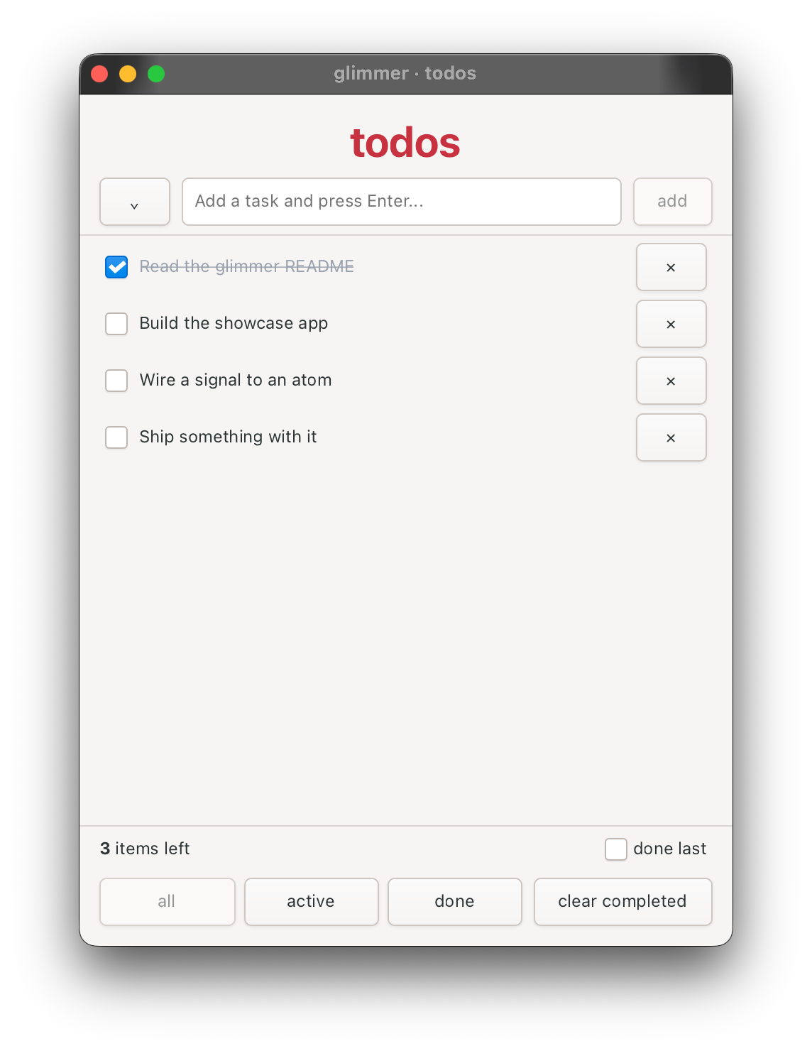
To prove the concept, I made glimmer which uses Reagent style reactive atoms to drive GTK components. A classic TodoMVC app illustrates how using a native UI toolkit is completely seamless from Jolt. The reactive data model has proven itself to be an extremely effective tool in ClojureScript, and wrapping GTK with a Reagent style API brings these same ergonomics to a native desktop environment giving us the best of both worlds. You get to work with reactive atoms and declarative component structure while using a fast native toolkit for rendering. The application ends up having a far smaller memory footprint than anything running in a Java virtual machine possibly could. And, of course, nREPL-driven development that we all know and love works here as well.
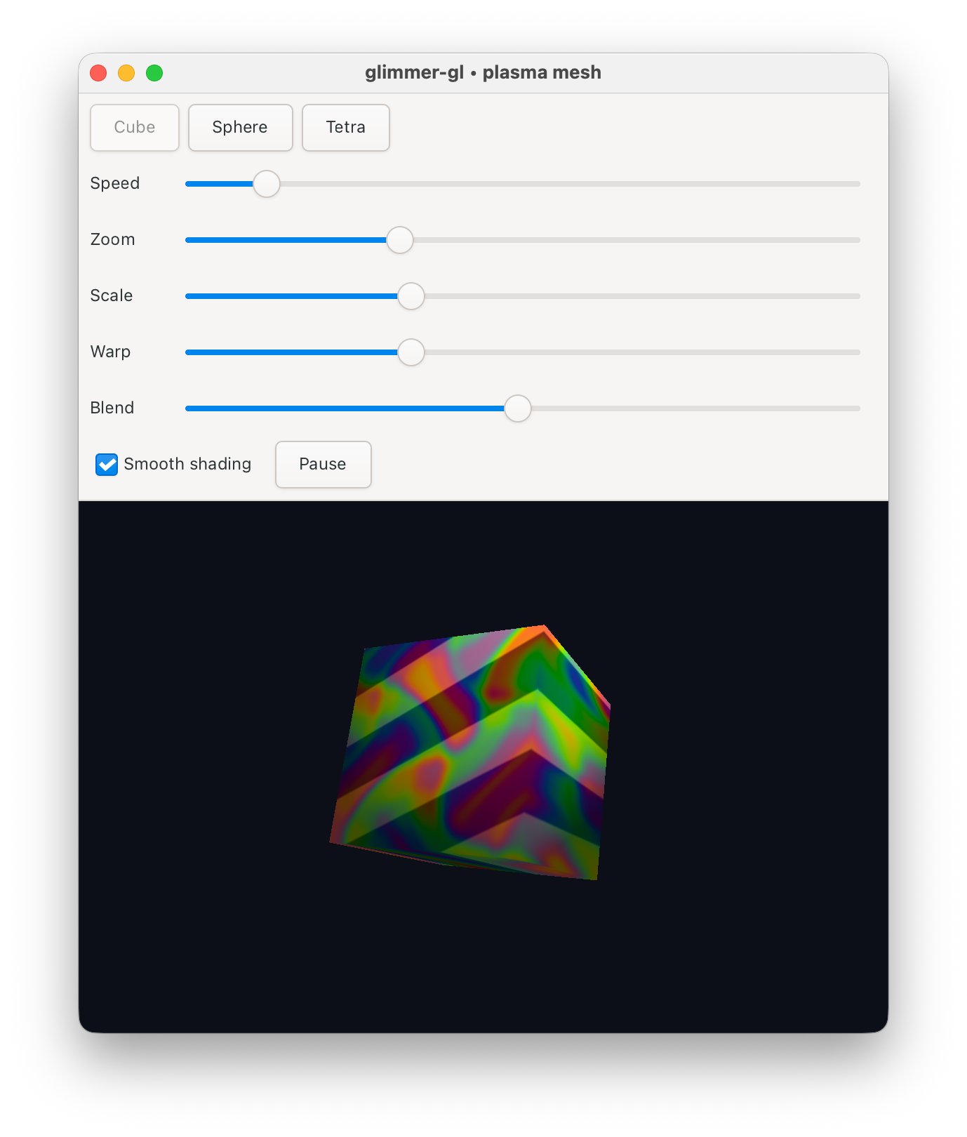
We can even take this further and create an OpenGL context from inside a GTK window with glimmer-gl. You can see how the reactive approach works seamlessly in this context here.
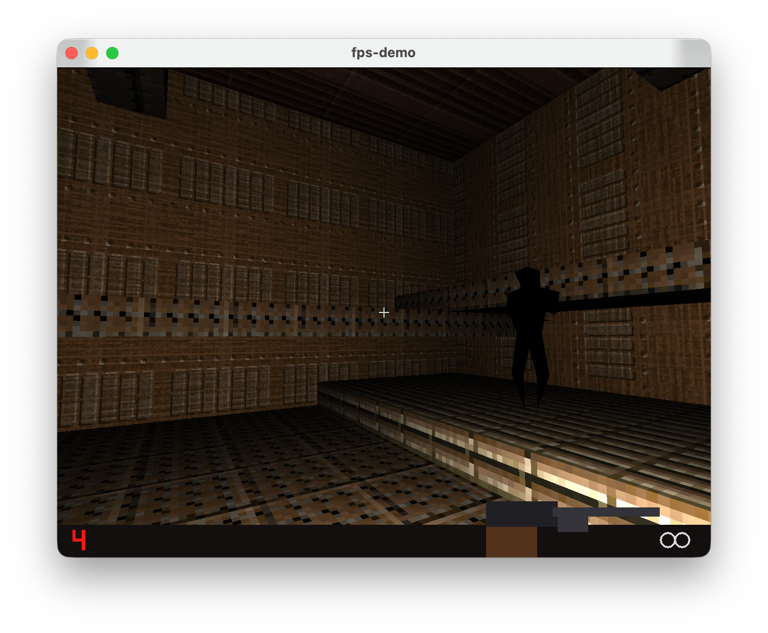
I even managed to get a whole Quake style FPS working on Jolt. Building reactive 3D scenes natively usually involves manually managing state mutations in a low level language. Driving an OpenGL pipeline directly from Clojure makes it easy to model complex visual state dynamically without sacrificing raw performance. You can build local graphics intensive tools that boot quickly and run smoothly. The developer experience stays entirely within the functional world of Clojure while the heavy lifting is done by a native library.
Deployment and Architecture
Deploying or distributing a Jolt app simply means building a binary for the target platform, and users don't need to have a JVM runtime installed on their machines to run it. In fact, you don't even need Chez Scheme installed to develop using Jolt because it produces its own joltc binary that's self contained. Another advantage is that it's possible to create a Jolt library that can be embedded in C, C++, or Rust projects where Jolt can provide a high level Clojure API and interactivity via nREPL on top of performant native code. This could be particularly appealing for projects with intensive graphics visualizations or even games using engines like Godot.
Architecturally, I've structured the compiler into three parts: there's a Clojure-in-Clojure compiler for the language itself, then there's a Scheme part consisting of the host layer and Java interop shims. As a stretch goal, I'm hoping to get a portable Clojure implementation out of the deal as well that could easily target different runtimes, for cases where JVM interop isn't needed. You can start with a minimally irreducible set of forms, and then grow the compiler itself like a seed, so that the host, whether Scheme or anything else, just needs to provide support for that minimal bootstrap code. However, moving functionality into Clojure layer can also be at odds with raw performance. A compromise here might be to have a portable Scheme layer which could target different implementations.
While Chez gives us a good overall target for Clojure, it makes a few architectural assumptions, like being able to write instructions to a section of memory and then execute that code, that do not hold for targets like WASM which considers such behavior a security concern. It would be useful to decouple the host layer from Chez and make it easy to port to different Scheme runtimes which would give us access to things like interactive development for WASM via Guile. Since host code is already separate from the core language implementation, there's some more refactoring that would be needed, but it wouldn't be difficult to isolate Chez specific bits, and build a general Scheme layer on top.
On Building with LLMs
At this point, it's worth discussing the fact that this project is built using LLM tools. The reality is that it simply would not be possible for me to take on a project of this scope otherwise. Writing a full Clojure port by hand would be a full time project. Using code generation tools actually made the effort tractable, and allowed me to prove the concept quickly. Of course, there are naturally concerns associated with this approach and how I ensure code quality when I'm not writing every line of code myself. So, I'd like to take a bit of time to discuss that here.
I'm going to make the argument that whether the code was written entirely by hand or produced by an LLM is the wrong thing to focus on. To see why, we have to consider how software development actually works at scale.
There's a view that code written by hand has to be more intentional, almost has to be by definition since it requires the maintainer to actually put it in there themselves. That's, of course, true but once a project grows past a certain size or it has multiple maintainers, nobody really has the totality of the code in their heads. So, any new code that's added is always done with limited understanding. Code being written by hand should not be equated with it expressing the intent faithfully; if that were the case, then we'd never have software bugs. Humans make mistakes all the time as is clearly evidenced by there being no lack of buggy code predating LLM use.
I'm also not intimately familiar with most of the code in the projects I've been maintaining over the years. Any code I've written even a few months ago might as well have been written by someone else. When I need to make changes, I read through the code and figure out what it's doing, and I rely on the test harness to make sure I don't introduce regressions.
It's simply not feasible for humans to keep the entirety of large projects in their heads all at once. When you're working on a project, you're constantly forgetting and relearning code as you go. And the situation is even worse for projects where multiple people work together where nobody knows what everyone else was thinking. We look at the code and try to build up sufficient context in our heads to make the necessary changes. When we misjudge that context or misunderstand existing code, then we end up making mistakes.
The way we judge whether projects are actually solid is by the level of specification and testing they have, the experience of the developers, and amount of usage they see in the wild. All of these same tools work just as well with LLM generated code as they do with code written by hand.
Farming out design decisions to the LLM without reviewing the output or doing proper testing will almost certainly produce low quality code, but that is no different from somebody just slapping some code together to make a kludge rather than really thinking through a problem. Working with LLMs does not mean farming out your thinking to the machine. What these tools actually do is automate the mechanical aspect of producing the code. Once it is written, you can read it, understand it, and change it as you would with any other code.
My process tends to be to give the agent focused tasks that implement a particular feature, then make commits for each, and review to see whether a feature has been implemented as I intended. This isn't all that different from a regular code review process which is known to be a good way to catch bugs.
I also have a high level of confidence in the code because it passes clojure-test-suite along with the tests for many existing Clojure libraries. The test corpus I built up for it ensures that the code does not regress when I make changes. And benchmarks I've set up ensure that performance does not regress. All these things combined give me as much confidence as I would have in a hand written project of the same scope. I would further argue that compilers are a particularly good target for LLMs because they are well specified by definition. You have data coming in, and corresponding data coming out. There is very little ambiguity regarding what constitutes correct behavior when you are implementing a language.
Conclusion
Ultimately, the quality of the project depends on the skill and interest of its maintainer rather than how the code was produced. If somebody has been writing code for many years, and has a proven track record of delivering quality projects, then it should be assumed that when they use a new tool like an LLM in their work, the output will be consistent with the standards that they have already demonstrated previously.
If you got this far then I hope you find the project interesting and you'll give Jolt a try. Things are fairly stable at this point, and compiler binaries are available via GitHub releases and homebrew. I set up a #jolt channel on Clojurians Slack for discussion and updates, and if you're interested in collaborating or discussing the direction of the project do drop by. Alternatively, if you run into any problems or have suggestions then feel free to open up issues or make pull requests on GitHub.